On Parallel Programming
By Pekka Enberg, 2020-01-31

Applications and services today are more data-intensive and latency-sensitive than ever before. Workloads in the cloud and the edge, such as AI/ML (deep learning), augmented reality, and autonomous vehicles, have to deal with high volumes of data with latency requirements in the order of microseconds or less. However, the stagnation of single-threaded performance forces system designers to turn their attention to parallel computing to support such latency and volume requirements.
Parallel computing has a long history in computer science. In fact, some of the very first computers having parallel architectures. For example, ENIAC, completed in 1945, could execute multiple independent instructions simultaneously [6]. Similarly, Whirlwind I, completed in 1951, was the first general-purpose supercomputer with parallel architecture [13]. However, since its inception in 1945, the sequential von Neumann architecture, remained the most influential computer architecture for decades In the 1970s, parallel computers become relevant again in supercomputers, which were designed around multiprocessors and vector architectures. But it wasn’t until 2006 with the breakdown of Dennard Scaling that parallel computer architectures started to become mainstream. As processor clock frequencies stalled, the industry was forced to move to multicore architectures, even on consumer devices.
Although parallel computing is increasingly important today, parallel programming techniques can be confusing to programmers that are more used to the sequential model. The goal of this blog post is to give an overview of the principles and concepts of parallel computing to help application and system designers to take advantage of parallelism in their designs.
Table of Contents
Concurrency and parallelism
Before we get into parallel computing and parallel programming, we need first to establish what parallelism is. You often hear the terms concurrency and parallelism used interchangeably, but they do not mean the same thing.
Concurrency is the composition of multiple computations into independent threads of execution [12]. For example, in POSIX, a process or a thread can be a unit of concurrency, and the Go programming language, a goroutine is a unit of concurrency. Concurrency is often needed to improve the utilization of the CPU. For example, if one thread of execution is waiting for an I/O to complete, another thread of execution can run the CPU. In fact, this concurrent use case of switching to another task while waiting for I/O by multiprogramming dates back to 1955 in academic literature [3].
Parallelism is the simultaneous execution of multiple computations [12]. For example, threads are a way to compose parts of an application to run concurrently, but when the threads run simultaneously on different CPUs, they’re executing in parallel. The main motivation for parallelism is to reduce latency and improve throughput. That is, parallelism is used to perform more work in less time by decomposing the problem into smaller pieces that can execute simultaneously.
The relationship between latency, throughput, and concurrency can be described with Little’s Law. In its most general form, Little’s Law states that, in a system that is in steady-state, the average number of items \(L\) in the system is the product of the average arrival rate \(\lambda\) and the average time \(W\) each item spends in the system [9]:
\(L = \lambda W\)
For computer systems, the same equation is often expressed as Little’s Law of High Performance Computing [2], which states that:
\(Concurrency = Latency \times Throughput\)
In other words, concurrency increases if either latency or throughput increases. Latency cannot be reduced beyond some threshold (because of physical constraints), which means that increasing throughput eventually increases concurrency. The increased concurrency inevitably reaches a point when parallelism is needed [11].
Limits of parallelism
Parallelization can reduce latency, but how much exactly?
There are two different theoretical answers, depending on whether the problem to be parallelized has a fixed size or not. Both answers build on the observation that a program has a serial part (not parallelizable) and a parallel part. The overall speedup depends on the amount of speedup from the parallelization but also the portion of the parallel part in the program.
Amdahl’s Law shows the theoretical speedup in latency when execution is parallelized for a fixed-size problem [1]. The law is defined as follows with \(N\) as the number of parallel execution units and \(P\) as portition of the program that can be parallelized:
\(Speedup = \frac{1}{(1-P)+\frac{P}{N}}\)
The following diagram illustrates Amdahl’s Law with speedup as the Y-axis and number of parallel execution units N in the X-axis:
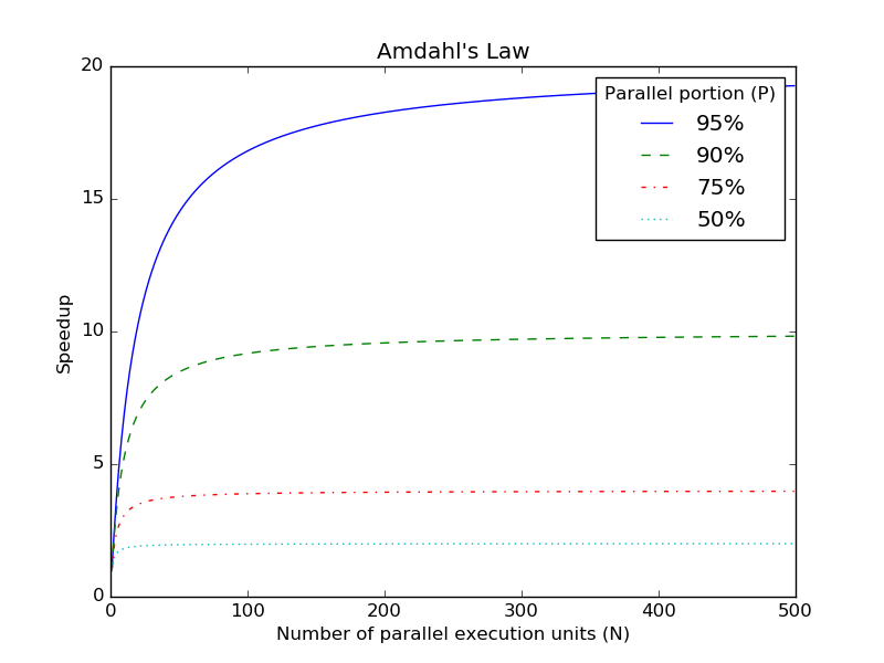
The different plot lines are varying the parallelizable portion P. A key observation from the diagram is that even with a relatively high parallelizable portion of 95%, the serial part of the program dominates execution, limiting the speedup to 20x even with a large number of parallel execution units.
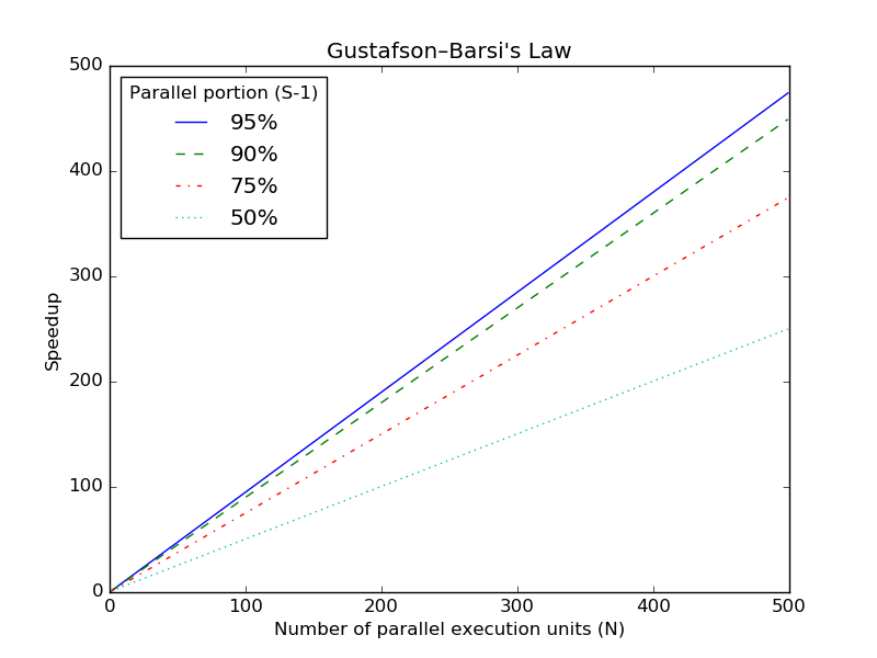
Amdahl’s law predicts a hard limit in speedup even with a small serial portion. However, in many workloads the problem is variable-sized where the size of the parallelizable problem scales with the number of processors. For example, a data processing job can be scaled to more and more processors processing more data. For such variable-sized problems, Gustafson—Barsi’ law defines the limits of speedup from parallelization.
Gustafson—Barsis’s Law shows the theoretical speedup in latency for problems that are variable-sized [7]. The law is defined as follows with \(N\) as the number of parallel execution units and \(s\) as the portion of the program that is serial:
\(Speedup = N+(1-N) \times s\)
The following diagram illustrates Gustafson—Barsi’s law with speedup as the Y-axis and number of parallel execution units N in the X-axis:
Sources of parallelism
Now that we understand what parallelism is and what are its limits, what are the different sources of parallelism that can be exploited?
Bit-level parallelism (BLP) is the parallelism present in every operation that manipulates a piece of data (for example, addition or subtraction). Although mostly a historical curiosity now, bit-level parallelism was a significant source of improved performance until the mid-1980s [4]. Increasing the width of the CPU datapath reduces the number of intermediate operations required to perform a full operation. For example, on an 8-bit CPU, adding two 32-bit integers required a total of four operations, whereas a 16-bit CPU requires two operations, and a 32-bit CPU requires only one.
Instruction-level parallelism (ILP) is the parallelism in program instructions that are independent of each that, which can, therefore, execute in parallel. The amount of ILP depends on the program. For example, the following program (written in RISC-V assembly) has ILP of 3, because each instruction is data independent:
    add     x1, x2, x3      // x1 := x2 + x3
    sub     x4, x5, x6      // x4 := x5 - x6
    mul     x7, x8, x9      // x7 := x8 * x9
However, the following program has ILP if only 1, because instructions depend on the result of the previous instruction making the data dependent:
    add     x1, x2, x3      // x1 := x2 + x3
    sub     x4, x5, x1      // x4 := x5 - x1
    mul     x6, x7, x4      // x6 := x7 * x4
A superscalar processor can exploit this ILP with instruction pipelining or multiple executions units, allowing the CPU to execute more than one instruction per cycle. Current out-of-order execution CPUs perform many optimizations at the microarchitectural level. For example, branch prediction is a critical optimization, where the CPU predicts the path a branch is going to take to keep the out-of-order execution units busy. To reduce false data dependencies at register level (access to the same register but without actual data dependency), CPUs perform register renaming to convert accesses to ISA registers into accesses to a larger set of internal registers. Similarly, to reduce memory dependencies, CPUs perform memory renaming to convert memory access to register access [14]. These microarchitectural optimizations are critical to exploiting instruction-level parallelism at execution time.
Thread-level parallelism (TLP) is the parallelism in the executing threads of a program. Threads that have no dependency on each other can execute in parallel on different CPU cores. Simultaneous multithreading (SMT) – also known as Hyper-Threading in Intel’s products – is a technique to transform TLP into ILP [10]. In CPU cores that support SMT, a physical core is divided into multiple logical cores, which share some functional units of the physical core. The rationale for SMT is to keep the functional units of a superscalar CPU busy.
Accelerator-level parallelism (ALP) is the parallelism of application tasks that are offloaded to different special-purpose accelerators that can compute specific tasks more efficiently than a CPU.
Request-level parallelism (RLP) is the parallelism of application request processing. For example, in a key-value store such as Memcached, clients send requests to a server to read or update a key in the store. The server executes these requests and sends responses to the clients. If these requests are independent of each other, they can be processed in parallel. Requests are independent if they do not use the same resources. Synchronization of a shared state is one of the biggest obstacles in parallel request processing.
Parallel computer architectures
Parallel computer architecture can be designed in several ways.
Flynn’s Taxonomy is largely a historical classification, but serves as a good starting point in understanding the trade-offs between different parallel computer architectures. As shown in Table 1, Flynn’s Taxonomy is essentially a classification based on how many instructions and data can be processed in parallel.
| Single Data | Multiple Data | |
| Single Instruction | SISD | SIMD |
| Multiple Instruction | MISD | MIMD |
SISD is a serial (no parallelism) computer architecture, which executes a single instruction that operates on a single data element at a time. The SISD architecture goes back to Von Neumann-style late-1940s computers such as EDVAC and EDSAC. Although a SISD architecture is serial from a programmer’s perspective, it can have parallel execution via pipelining and superscalar execution as a performance optimization.
MISD is a parallel computer architecture, which executes multiple instructions on the same data stream in parallel. This type of parallel architecture is not very common but can be useful, for example, for fault tolerance, where multiple redundant instructions are working on the same data.
SIMD is a parallel computer architecture, which executes the same instruction on multiple data streams in parallel. These architectures exploit data-level parallelism while retaining the serial flow of control by executing a single instruction at a time. Examples of SIMD architecture are the Advanced Vector Extensions (AVX) and Streaming SIMD Extensions (SSE) instructions sets in the x86 machine architecture. SIMT (single instruction, multiple threads) extends the SIMD model with multithreading. The SIMT model is used by many GPU architectures today.
MIMD is a parallel computer architecture, which executes a single instruction on a single data element per processor, but has multiple processors. That is, a MIMD architecture is the SISD architecture turned into a parallel computer by multiplying the number of processing units (multicore). SPMD (single program, multiple data) is a subcategory of MIMD that often refers to a message passing architecture over distributed memory.
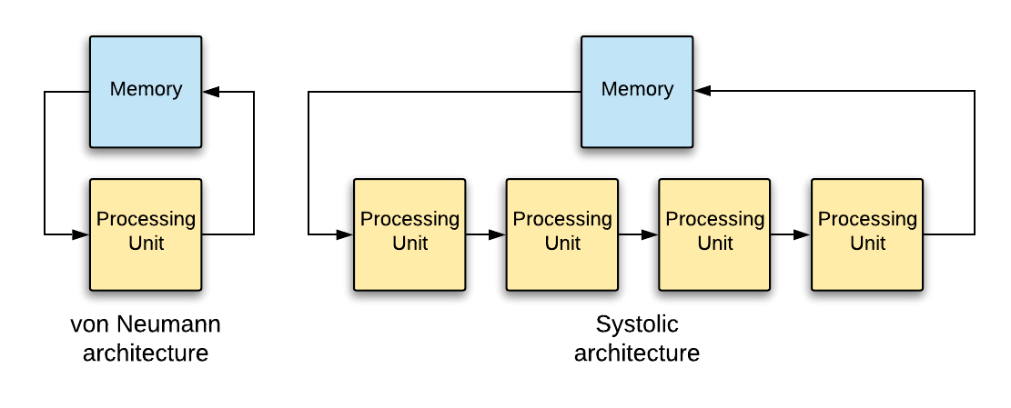
Systolic architecture is a parallel computer architecture, where data flows through a network of processing units. Figure 1 shows the differences between von Neumann and systolic architectures. In systolic architectures, processing units forward intermediate results to the next processing unit directly, without going through the main memory. With DRAM access speeds at ~100 ns and SRAM access at ~10 ns, eliminating main memory access for intermediate results can improve processing performance significantly. Systolic architectures were invented in 1978 by Kung and Leiserson [8], but the techniques dated back to the Colossus Mark 2 (developed in 1944). Today systolic architectures are used in Google’s TPU, an energy-efficient accelerator for neural network computations, usually written in TensorFlow.
Applications and parallelism
Parallelism can reduce latency and improve throughput, but how can applications take advantage of parallelism?
From an application architecture point of view, the decision on what to share between processing units has a huge impact.
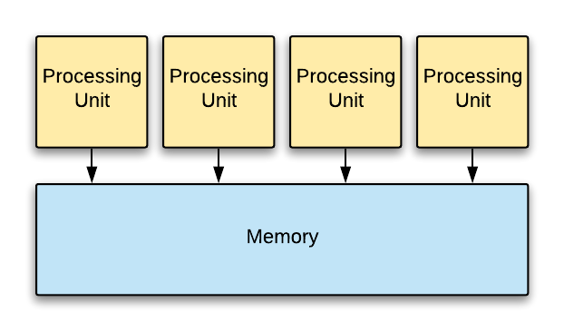
In the shared-everything approach, shown in Figure 4, parallel threads of execution can access all the hardware resources. For example, in the POSIX model, a process can spawn multiple threads that access the process memory address space, kernel state (e.g, filesystem), and hardware resources. The sharing of resources maximizes hardware utilization but requires synchronization between the threads for consistency. Locking primitives can be used for synchronization, but the scheme can limit scalability to multiple processors because of lock contention.
In the shared-nothing approach, shown in Figure 5, resources are partitioned between processors to eliminate the overheads of thread synchronization. For example, system memory is divided into partitions, and only one processor accesses a single partition. The partitioning allows each processor to execute independently without having too coordinate accesses with other processors (for example, using locking). Of course, in many applications, there is also a need for inter-processor communication to distribute work, access remote resources, and so on. The communication channels require coordination between the communicating processors, but there are efficient implementation techniques such as lockless, single-producer, single-consumer (SPSC) queues to do that.
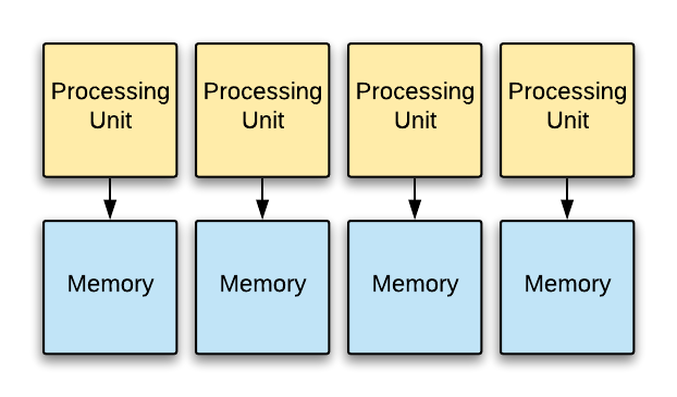
One disadvantage of the shared-nothing approach is that not all processors are utilized for skewed workloads. For example, if the keyspace is partitioned between processors in a key-value store, clients that access only a subset of the keys may not be able to utilize all the cores. The application-level partitioning scheme is critical to the shared-nothing approach to take advantage. Another challenge in the shared-nothing approach is request steering. Requests that arrive from the network land on one of the NIC queues, which is processed by a processor. However, that request might access a data element that resides on the partition of another processor. This requires applications to steer requests to a different processor, which can have significant overheads.
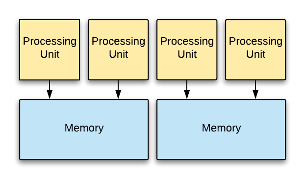
The shared-something approach, shown in Figure 6 is a hybrid between the shared-everything and shared-nothing approaches. Application partitions system resources, but allows more than one processor to access each partition. That is, system resources are partitioned between a group of processors rather than a single processor. Within each partition, processors must coordinate accesses with each other, but each group of processors can execute independently.
From a programming model point of view, the decision between task and data parallelism is also critical.
Task parallel programming model focuses on parallelization of computation. For example, the Fork/Join model is a task-parallel approach that application to fork execution of the program (parallel execution) and eventually join the different parallel executions (synchronization). The implementations of the Fork/Join model usually use light-weight threads such as fibers for execution on a single computer. Cilk programming language and OpenML are examples of task-parallel systems.
Data parallel program model, in contrast to the task parallel model, focuses on parallelization of data access. For example, in the MapReduce model, the programmer defines two functions: a map function that takes a key-value pair as its input and produces a set of intermediate key-value pairs and a reduce function that merges the intermediate values by key [5]. A program that has been decomposed using map and reduce functions can be automatically parallelized. From a theoretical perspective, MapReduce can be classified as is an SPMD architecture.
Summary
Parallel programming is important when designing high-performance systems today. Theoretical frameworks such a Little’s Law, Amdahl’s Law, and others can help in making design decisions that lend themselves to parallelism. Understanding and exploiting the different sources of parallelism across the hardware/software stack are the key for high-performance implementations. But perhaps most importantly, it is essential to select an architecture and a programming model, which maximizes your chances of exploiting parallelism for your specific workload.
Updates
- 2020-02-13: Clarify the difference between Amdahl’s Law and Gustafson—Barsi’ Law as per a reader comment on lobste.rs.
Acknowledgments
Thanks to Duarte Nunes and Jussi Virtanen for their valuable feedback on this blog post.
References
[1] Amdahl, G.M. 1967. Validity of the Single Processor Approach to Achieving Large Scale Computing Capabilities. Proceedings of the April 18-20, 1967, Spring Joint Computer Conference (Atlantic City, New Jersey, 1967), 483–485.
[2] Bailey, D.H. 1996. Little’s Law and High Performance Computing.
[3] Codd, E. 1962. Multiprogramming. Advances in Computers. 3, (1962), 77–153.
[4] Culler, D. et al. 1998. Parallel Computer Architecture: A Hardware/Software Approach. Morgan Kaufmann.
[5] Dean, J. and Ghemawat, S. 2008. MapReduce: Simplified Data Processing on Large Clusters. Communications of the ACM. 51, 1 (2008), 107–113.
[6] Gill, S. 1958. Parallel Programming. The Computer Journal. 1, 1 (1958), 2–10.
[7] Gustafson, J.L. 1988. Reevaluating Amdahl’s Law. Communications of the ACM. 31, 5 (1988), 532–533.
[8] Kung, H.T. 1982. Why systolic architectures? Computer. 15, 1 (1982), 37–46.
[9] Little, J.D. 2011. Little’s Law as Viewed on Its 50th Anniversary. Operations research. 59, 3 (2011), 536–549.
[10] Lo, J.L. et al. 1997. Converting Thread-Level Parallelism to Instruction-Level Parallelism via Simultaneous Multithreading. ACM Transactions on Computer Systems (TOCS). 15, 3 (1997), 322–354.
[11] Padua, D. 2011. Encyclopedia of Parallel Computing. Springer Publishing Company.
[12] Pike, R. 2012. Concurrency is not Parallelism.
[13] Sterling, T. et al. 2018. High Performance Computing: Modern Systems and Practices. Morgan Kaufmann.
[14] Tyson, G.S. and Austin, T.M. 1999. Memory Renaming: Fast, Early and Accurate Processing of Memory Communication. International Journal of Parallel Programming. 27, 5 (1999), 357–380.